Sampling from Any Distribution
tl;dr: this post will be a (somewhat) deep-dive into implementing code which samples from any arbitrary probability distribution.
Motivation
Lately I've been really interested in probabilistic programming. As I'm learning, I hope to collect interesting ideas and present them here.
A probabilistic program, in its simplest form, is just a program where some of its variables are stochastic. Probabilistic programming languages come with tools to take this program and do interesting things, such as fixing the values of certain stochastic variables and querying for the inferred values of other variables.
def model(is_cont_africa, ruggedness, log_gdp):
    a = pyro.sample("a", dist.Normal(0., 10.))
    b_a = pyro.sample("bA", dist.Normal(0., 1.))
    b_r = pyro.sample("bR", dist.Normal(0., 1.))
    b_ar = pyro.sample("bAR", dist.Normal(0., 1.))
    sigma = pyro.sample("sigma", dist.Uniform(0., 10.))
    mean = a + b_a * is_cont_africa + b_r * ruggedness + b_ar * is_cont_africa * ruggedness
    with pyro.plate("data", len(ruggedness)):
        pyro.sample("obs", dist.Normal(mean, sigma), obs=log_gdp)
(Example of a statistical model encoded as a probabilistic program. Credit: pyro.ai docs)
Probabilistic programs are a convenient way to express statistical models. What I'm particularly excited about, though, is viewing probabilistic programming as a new paradigm, fusing traditional programming and machine learning. Through this lens, we might see a probabilistic program as an explicit representation of which parts of a system encode concrete constraints, and which parts contain parameters to be learned. I'm excited to learn more about the uses of probabilistic programming in building intelligent agents which reason in a safe-by-design way (I'm thinking in particular of the work of Ought).
But I'm getting ahead of myself: for now, I just want to think about the most basic building block of a probabilistic program. Consider this statement, in an imaginary Python-based probabilisitic programming language:
x = sample(Normal(mean=0, std=1))
In words, "let x be a random variable, drawn from a normal distribution with mean 0 and standard deviation 1". How is it implemented? How would we "run" this program and get an actual value (or several values) for x?
Ideally, there would be nothing special about Normal: we should be able to implement our own probability distribution by specifying a probability density function, for example:
@dataclass
class Normal:
mean: float
std: float
@cached_property
def beta(self):
return self.std ** -2
def pdf(self, x):
exponent = -2 * self.beta * (x - self.mean) ** 2
multiplier = self.beta / np.sqrt(2 * np.pi)
return multiplier * np.exp(exponent)
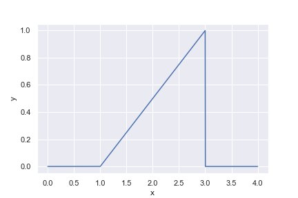
@dataclass
class Triangle:
"""
A probability distribution where probability density increases
linearly from `l` to `u`, and is 0 everywhere else.
"""
l: float
u: float
def pdf(self, x):
if not self.l < x < self.u:
return 0
return 2 * (x - self.l) / (self.u - self.l) ** 2
In the remainder of this blog post, I'll implement all the building blocks for performing this sampling.
I'll be omitting boilerplate such as imports and protocol definitions, but you can find the complete Jupyter notebook here.
(Pseudo-)random number generators
The first step towards drawing a random sample from a given distribution, is just drawing some kind of random number from somewhere.
If we need proper random numbers, we'd need some source of randomness in the real world. For the purposes of this blog post, I'll stick to a pseudorandom number generator. These work by, starting with a seed, producing a deterministic sequence of numbers which look pretty random.
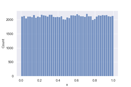
In particular, the Mersenne Twister algorithm, used by Python's random module produces values which are uniformly distributed between 0 and 1.
sns.histplot(
    data={"x": [random.random() for _ in range(100_000)]},
    x="x",
)
Transforming the Uniform Distribution
Right, so we have a way to get samples that are uniformly distributed. Are there any easy ways to transform that distribution into a different one?
To start with, we can easily scale or translate to get samples drawn from Uniform(l, u) for arbitrary lower and upper bounds l and u, as follows:
@dataclass
class UniformSampler:
    lower: float
    upper: float

    def draw(self) -> float:
        width = self.upper - self.lower
        return self.lower + random.random() * width

def plot_pdf(sampler: Sampler, n=1_000_000):
    samples = [sampler.draw() for _ in tqdm(range(n))]
    sns.kdeplot(data={"x": samples}, x="x", bw_adjust=0.5)

plot_pdf(UniformSampler(5, 10))

The PDF of Uniform(5, 10) is the same as Uniform(0, 1) but stretched horizontally and squished vertically. In general, however, there's no easy way of transforming a uniform sample into a sample drawn from another distribution.
Rejection Sampling
Although we can't simply transform a single draw from a uniform distribution into any other, we can if we're allowed to take multiple draws. Here's how it works, supposing we want to draw from a distribution $D$:
- Take a uniform sample $x$ over $\left[l, u\right]$, where $l$ and $u$ are bounds within which the vast majority of $D$'s probability mass is found
- Calculate $t = p_{X ~ D}(X=x)$
- Take a uniform sample $y$ over $[0, 1]$
- If $t > y$, output $x$. Otherwise, repeat from step 1.
@dataclass
class RejectionSampler:
    dist: Distribution
    lower: float = -1000
    upper: float = 1000

    @cached_property
    def x_sampler(self):
        return UniformSampler(self.lower, self.upper)

    @cached_property
    def y_sampler(self):
        return UniformSampler(0, 1)

    def draw(self) -> float:
        while True:
            x, y = self.x_sampler.draw(), self.y_sampler.draw()
            if self.dist.pdf(x) > y:
                return x

sampler = RejectionSampler(Normal(0, 1), lower=-20, upper=20)
plot_pdf(sampler, n=100_000)
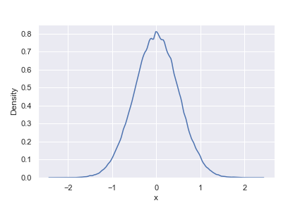 As you can see, this algorithm works perfectly. There are 2 remaining problems however.
Firstly, we had to pick the bounds -20 and 20 to draw samples. For this particular distribution we could pick those numbers manually, but ideally we wouldn't have to: either they could be picked automatically, or (as would happen in practice for the Normal distribution) the sampling algorithm could behave differently at the tails, allowing us to actually sample from the whole distribution. I won't explore this point further in this blog post.
Secondly, this method is very computationally expensive. Of course, I'm using a lot of plain Python for pedagogical purposes which could be easily vectorised with numpy etc., but there is also a lot of computation inherent in the algorithm.
To visualise this, consider the plot below:
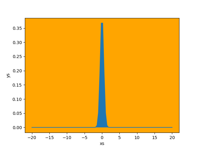
Every loop in the rejection sampling algorithm is like picking a point randomly from this whole plot. If that point happens to lie within the blue region, then we accept it - otherwise we have to pick a new point. Since the overwhelming majority of space is orange, it's clear that for each accepted sample there are many, many rejections.
More efficient distribution sampling
Without going into too much detail in this blog post, I want to convey the idea of how we can make rejection sampling more efficient.
The first insight is to divide the $XY$-plane into several regions which have equal probability mass (i.e. have the same blue area within them), then we can save a lot of effort by first randomly choosing a region, then sampling from that region.
The second insight is to note that, if we design these regions carefully and do enough pre-calculation, we might not even need to consult the PDF to know whether to reject or accept points within that region. Consider the following division of half a Normal distribution:
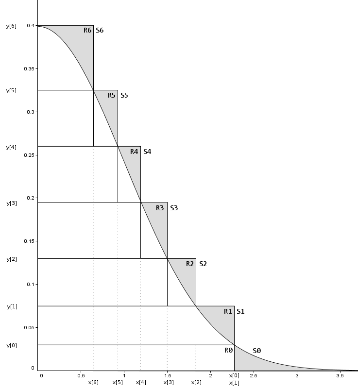
Image credit: https://heliosphan.org/zigguratalgorithm/zigguratalgorithm.html
Imagine we pick one of the middle rectangles. If we sample some $x$ value from within that rectangle's bounds, and our $x$ value turns out to be inside the grey line, then we don't need to evaluate the PDF, we can just accept that value. Since (for this distribution) most of the probability mass is inside the grey lines, this eliminates a bunch of our PDF evaluations. Hooray!