AI Disclosure: I used ChatGPT to help me generate the plots for this blog post, but all the words are my own.

In this blog post, I'd like to continue my exploration of sampling algorithms.

I'm particularly interested in general-purpose sampling algorithms, i.e. algorithms that take as input a probability density function and output a sample of that distribution. Here's what I'm looking for in code:

def pdf(x: float) -> float: ...

sampler = Sampler(pdf)

sampler.draw()

As a reminder, in the last post I talked about (Naive) Rejection Sampling, which is about the simplest imaginable algorithm for sampling from a distribution:

1. Specify lower and upper bounds $l, u$ for the values we will sample (for now, let's just treat these as hyperparameters)
2. Uniformly choose some $x \in [l, u]$ and some $y \in [0, 1]$.
3. Check if $pdf(x) \le y$. If so, return $x$. If not, repeat from step 2.

Though this will give us accurate samples, it's extremely inefficient, and there's a really mean tradeoff between how wide we set our bounds and how likely a sample is to be rejected.

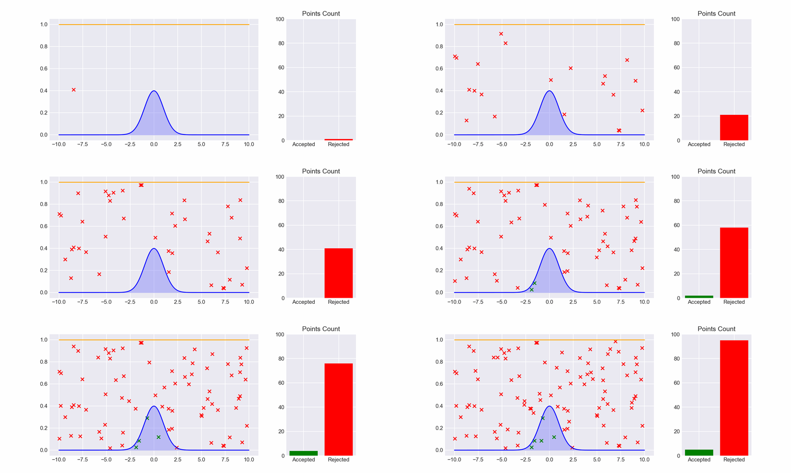We can of course do much better, and in some cases without an awful lot of extra work.

Side note: there's no need to normalise

In general, for the following algorithms, we don't need to make sure our pdf has a total area of 1. In all these algorithms, we are just interested in sampling from a particular x-value in proportion to the pdf at that point, so it will work just fine even if the area is $\neq 1$.

Optimising the Envelope

Looking at naive rejection sampling, there's a lot of samples drawn from areas in the rectangle that are obviously going to fail: for example, the maximum value of the pdf is around 0.4, so any time we sample from the upper half of the rectangle that sample will always fail.

We call the rectangle from which we're sampling the envelope, and there's lots of improvements we can make to how we generate the envelope that can significantly improve the efficiency of sampling.

What is the envelope?

The envelope is some function $env$ we actually sample points from, which we then reject or accept to get samples of the function we're interested in. In order to do this job, we need 2 things from the envelope:

1. We need to be able to sample accurately and efficiently from the envelope
2. The envelope function needs to always be bigger than our target function $f$

For naive rejection sampling, we've chosen the dumbest possible envelope function:

$$ env(x) = \begin{cases} 1 \text{ if } x \in [l, u] \ 0 \text{ otherwise} \end{cases} $$

One easy way to make this more efficient is to move the envelope down to the top of our target function curve, i.e.

$$ env(x) = \begin{cases} \max(f) \text{ if } x \in [l, u] \ 0 \text{ otherwise} \end{cases} $$

If we do this, our efficiency already shoots up:

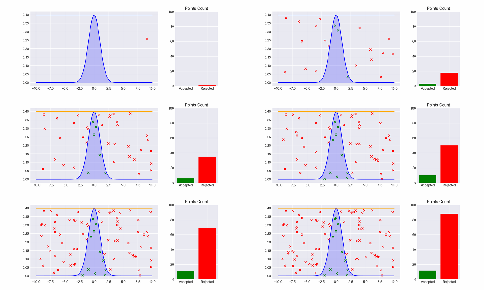
Still pretty inefficient though, and we've breezed past how we figured out the maximum of our target function. We can do better.

Sampling from more complex envelope shapes

So far our envelope has been just a rectangle, which is very easy to sample from: just take 2 uniform samples. However it's also not very expressive, and we'll struggle to really improve our efficiency on any target function that doesn't look like a rectangle itself.

A better class of envelope functions is piecewise linear functions. We have 2 problems to solve before we can use piecewise linear envelopes:

1. How do we sample from a piecewise linear function?
2. How do we find a piecewise linear envelope for our target function?

The first problem is somewhat easier, so let's start there.

A composable library of functions for exact sampling

We can build up to sampling piecewise linear functions by starting with some simpler building blocks. First of all, consider "triangular functions", i.e. line segments starting or ending at 0. Here's some code that samples from such a triangular function:

class TriangleSampler(Sampler):
    def __init__(self, x1, y1, x2, y2):
        assert y1 == 0 or y2 == 0, "One of y1 or y2 must be 0"
        domain = (x1, x2)
        slope = (y2 - y1) / (x2 - x1)
        self.base = x2 - x1
        self.height = max(y1, y2)
        total_area = 0.5 * self.base * self.height
        super().__init__(total_area, domain)
        self.x1, self.y1, self.x2, self.y2 = x1, y1, x2, y2
        self.slope = slope

    def f(self, x):
        if self.x1 <= x <= self.x2:
            return self.slope * (x - self.x1) + self.y1
        else:
            return 0

    def draw(self):
        r = random.uniform(0, self.total_area)
        if self.y1 == 0:
            return self.x1 + math.sqrt(2 * r / abs(self.slope))
        else:
            return self.x2 - math.sqrt(2 * (self.total_area - r) / abs(self.slope))

The exact formula of the draw method comes from the fact that, to sample from a PDF $f$, we can find the $x$ such that the CDF $F(x) = r$, where $r$ is uniformly distributed over $[0, 1]$. If our function $f$ is only nonzero in the domain $[x_1, x_2]$, then

$$ F(x) = \int_{x_1}^x f(z) dz $$

In our case, $f(z) = \frac{y_2 - y_1}{x_2 - x_1} (z - x_1) + y_1$, so plugging that in we get

$$ F(x) = \int_{x_1}^x \frac{y_2 - y_1}{x_2 - x_1} (z - x_1) + y_1 , dz = r $$

I won't bore you with expanding, integrating and solving the resulting quadratic equation for $x$, but what you get is exactly what we see in the draw method above.

sampler = TriangleSampler(x_1=0, y_1=2, x_2=1, y_2=0)
visualize_sampler(sampler, 100_000, 100

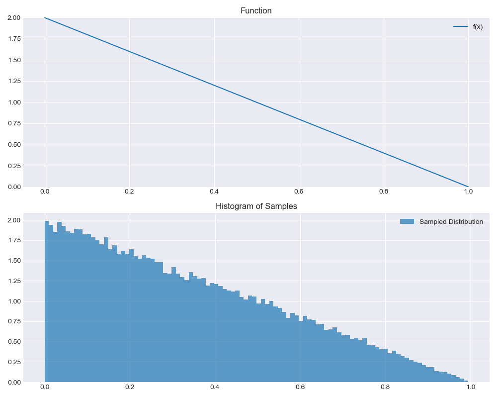
Next, let's write a sampler that takes another function and translates it on the y-axis.

class TranslatedSampler(Sampler):
    def __init__(self, sampler, h):
        self.sampler = sampler
        self.h = h
        self.domain = sampler.domain
        # Total area is the sum of the original area and the area of the added rectangle.
        self.added_area = (self.domain[1] - self.domain[0]) * h
        self.total_area = sampler.total_area + self.added_area

    def f(self, x):
        return self.sampler.f(x) + self.h

    def draw(self):
        # Decide whether to sample from the original distribution or the added rectangle.
        if random.uniform(0, self.total_area) < self.added_area:
            # Sample uniformly from the domain.
            return random.uniform(self.domain[0], self.domain[1])
        else:
            # Sample from the original distribution.
            return self.sampler.draw()

This one is very straightforward: to sample from the translated function, we either sample from the original function, or we sample (uniformly) from the rectangle we just added at the bottom. We choose which of the 2 to sample from in proportion to their areas.

Now we can combine our TriangleSampler and TranslatedSampler to sample from any line segment:

def create_segment_sampler(p1, p2):
    """Create a sampler for a segment between points p1 and p2."""
    x1, y1 = p1
    x2, y2 = p2

    base_height = min(y1, y2)
    triangle_sampler = TriangleSampler(x1, y1 - base_height, x2, y2 - base_height)
    if base_height > 0:
        return TranslatedSampler(triangle_sampler, base_height)
    else:
        return triangle_sampler

sampler = create_segment_sampler((1, 3), (2, 5))
visualize_sampler(sampler)

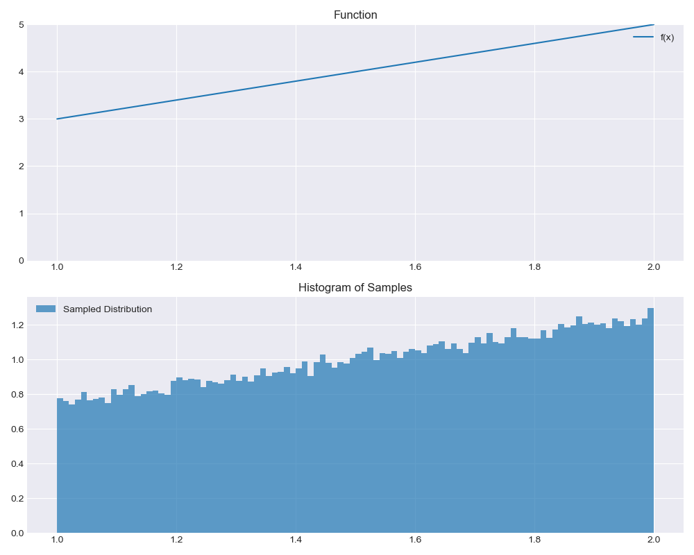
Finally, we'll write a sampler that horizontally composes 2 samplers:

class ComposedSampler(Sampler):
    def __init__(self, samplers):
        # Check if the domains of the samplers align properly
        for i in range(len(samplers) - 1):
            assert samplers[i].domain[1] == samplers[i + 1].domain[0], "Domains of consecutive samplers must align."

        self.samplers = samplers
        # Calculate the total area of all samplers combined
        self.total_area = sum(sampler.total_area for sampler in samplers)
        # The domain of the composed sampler
        self.domain = (samplers[0].domain[0], samplers[-1].domain[1])

    def f(self, x):
        # Find the appropriate sampler for the given x and use its f function
        for sampler in self.samplers:
            if sampler.domain[0] <= x <= sampler.domain[1]:
                return sampler.f(x)
        return 0

    def draw(self):
        # Choose a sampler based on their relative areas
        r = random.uniform(0, self.total_area)
        cumulative_area = 0
        for sampler in self.samplers:
            cumulative_area += sampler.total_area
            if r <= cumulative_area:
                return sampler.draw()

Similar to the TranslatedSampler, the draw method works by drawing a sample from one of the sub-samplers, choosing a sub-sampler in proportion to the total area under its function.

Using these building blocks, we can finally write a function that builds a sampler for any piecewise linear function:

def piecewise_linear_sampler(points):
    samplers = [create_segment_sampler(points[i], points[i+1]) for i in range(len(points) - 1)]
    return ComposedSampler(samplers)

sampler = piecewise_linear_sampler([
    (0, 1),
    (3, 2),
    (4, 8),
    (5, 6),
    (6, 6),
])
visualize_sampler(sampler)

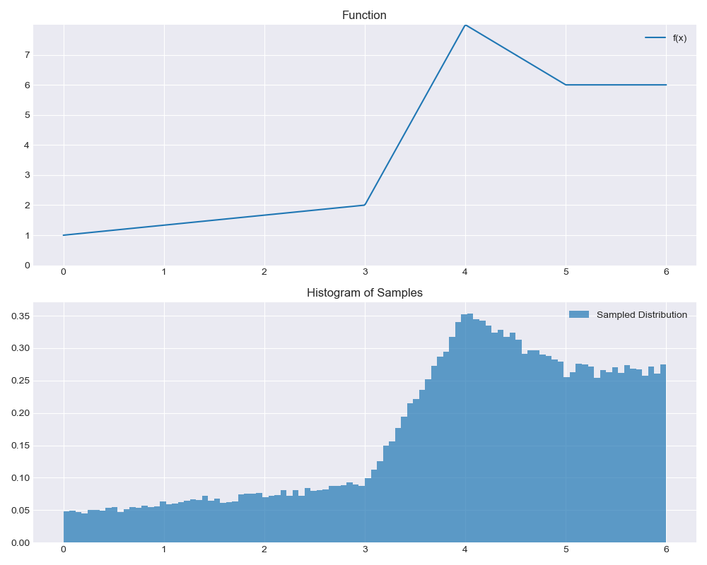
Great! Now we can sample from piecewise linear functions. What now?

Fitting envelopes to functions

As a reminder, we're trying to improve our rejection sampling algorithm, by reducing the number of samples that need to be rejected. We have developed a method of sampling from piecewise linear functions, but now we need to find a way of choosing a piecewise linear function to use as the envelope for our function to sample.

It's important that the envelope is always greater than the target function, since otherwise there will be parts of the original function that we don't sample correctly. However, it's pretty difficult to fit such an envelope to an arbitrary function.

Naive piecewise linear envelope

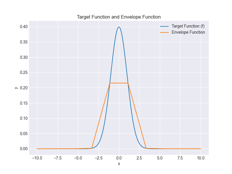
As a first pass, we could simply pick $n$ points on our line and draw straight lines between them. For these examples, I'll use a Gaussian, with $n=10$ for clarity.

This doesn't work, because where the function is concave, we end up underestimating it - very bad!

Using tangents instead of joining up lines

OK, how can we avoid underestimating the middle of the gaussian curve? Instead of simply joining up points on the function, we could try taking tangents to our function at various points, and joining those up. Doing this gives us the following "envelope":

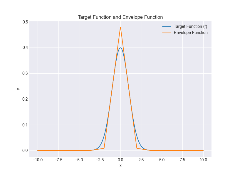
This works better in the middle, but we're now underestimating the tails. Perhaps there's a way we can combine both?

Combining these two approaches

It turns out that taking the maximum of these 2 approaches gives us a decent estimate:

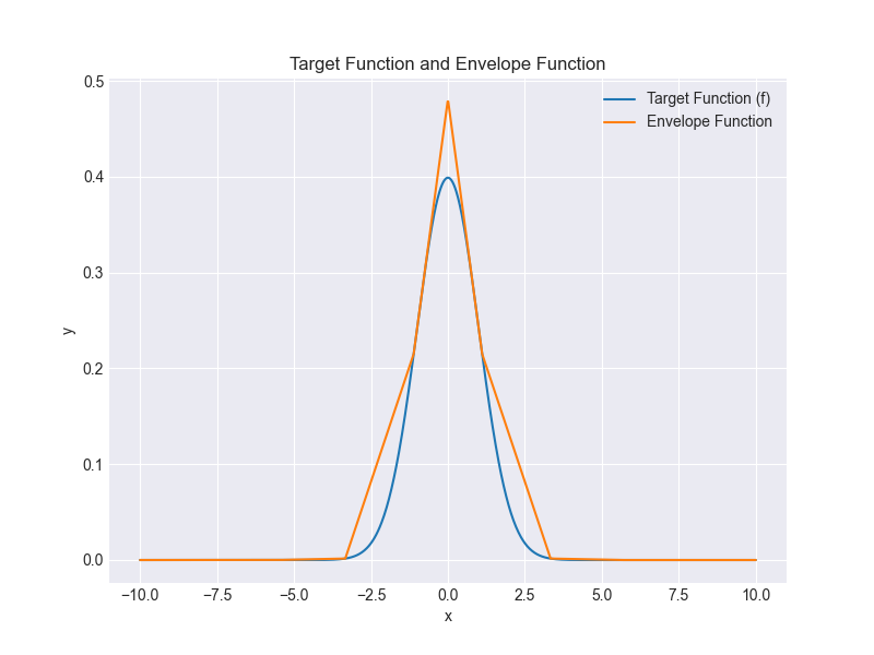
Of course, increasing the number of points (to 25) for the envelope will improve the fit:

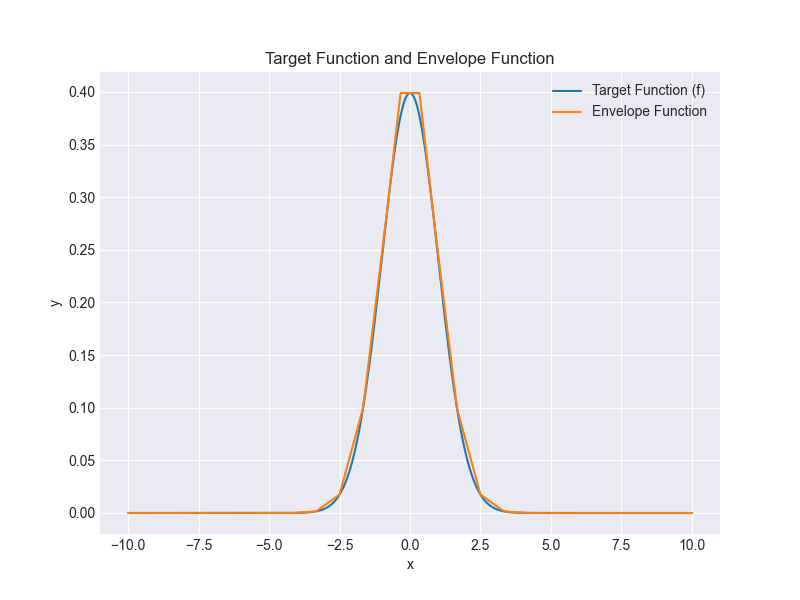
This envelope fitting algorithm is designed to be pragmatic, rather than theoretically perfect - it won't always be greater than the target function, but as long as we use enough points to generate the envelope, we should be OK.

In the literature, these sampling algorithms are usually referred to as "adaptive rejection sampling", and the envelope is continually improved as more points are sampled from the original function. For the purposes of this blog post (and because it's easier to plot), I'll stick with fitting the envelope once at the beginning.

Putting it all together

Now that we can fit envelopes to functions, and we can sample from those envelopes, let's put all the pieces together to see how rejection sampling fares:

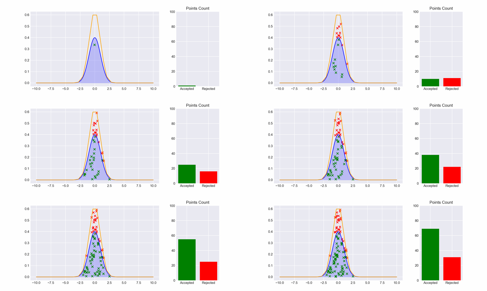So much better!

Links

You can find all the code for this blog post in this notebook.